Nanoparticle tracking analysis (NTA) reports two things no other routine sizing technique gives you directly: a particle-by-particle hydrodynamic diameter and an absolute particle concentration, both derived from tracking individual particles’ Brownian motion on video. Use it when you need number-weighted size distributions, need to detect minor subpopulations or aggregates hidden inside a bulk sample, or need a real concentration figure rather than a relative intensity signal. The technique works reliably across roughly 10 to 1,000 nanometers, though the exact window depends on your instrument and sample. Its main weaknesses are operator dependence and reduced sensitivity at the smallest end of that range.

---

TL;DR:

• NTA provides true particle-by-particle sizing and concentration data, but sensitivity depends on refractive index contrast and optical setup.
• The effective size detection window ranges from about 10 to 1,000 nanometers, with accuracy influenced by particle composition and instrument calibration.
• It’s preferable to run multiple video replicates—ideally 15 to 25—to achieve reliable concentration measurements and reduce variability.
• Operator-dependent adjustments like detection threshold and camera settings can cause significant result variation; strict SOP adherence is essential.
• NTA reliably supports extracellular vesicle, lipid nanoparticle, and protein aggregation research, especially when combined with orthogonal validation methods.

---

Table of Contents

• How Does Nanoparticle Tracking Analysis Work?
• NTA vs DLS: Which Should You Use?
• What Instrument Modes Does NTA Offer?
• What Sample Prep and Settings Give Reproducible Results?
• How Should You Interpret and Report NTA Data?
• Where Does NTA Add the Most Value?
• What Common Mistakes Undermine NTA Data?
• Mayflowerbio’s Nanoparticle Tracking Analysis Services
• A Minimum Reporting Standard Worth Enforcing
• Get Reproducible NTA Data Without Building It In-House
• Sources
• FAQ

How Does Nanoparticle Tracking Analysis Work?

NTA works by filming particles as they move randomly through a liquid, then converting that motion into a size measurement using physics that has been settled since 1905. A laser illuminates the sample in a thin optical path, particles scatter light, and a camera captures a video of the resulting flickering points. Software then does the real work: detecting each particle in every frame, linking those detections into a trajectory across frames, and calculating how far each particle wanders over time.

That wandering, known as Brownian motion, is not random noise to be filtered out. It is the measurement itself. Smaller particles get knocked around by solvent molecules more violently and diffuse faster; larger particles diffuse more slowly. The relationship between diffusion speed and particle size is described by the Stokes–Einstein equation, which relates the diffusion coefficient to hydrodynamic diameter through temperature and solvent viscosity. Software calculates the mean squared displacement for each tracked particle, plugs it into that equation, and outputs a diameter, one particle at a time.

Concentration comes from a separate calculation. The instrument knows the volume of liquid it is imaging in any given frame, based on the dimensions of the flow cell or cuvette and the depth of the optical field. Count how many distinct particles appear across a known number of frames, divide by that sampling volume, and you get particles per milliliter. This is why NTA concentration data is only as good as the calibration of that sampling volume and the consistency of particle detection settings.

Several variables shift where the detection range actually sits for a given setup:

• Refractive index contrast between particle and solvent: low-contrast particles (some liposomes, dilute protein aggregates) scatter less light and are harder to detect at small sizes.
• Laser wavelength: shorter wavelengths scatter more efficiently off smaller particles, extending the lower detection limit.
• Optical configuration: numerical aperture and camera sensitivity determine how faint a scattering event the system can still resolve as a real particle.
• Particle composition: metallic and high-density nanoparticles scatter far more strongly than organic vesicles of the same size, which changes the effective concentration range where accurate counting is possible.

Instrument detection range: Published characterization work puts the practical NTA sizing window at roughly 10 to 1,000 nanometers, though real-world performance at either extreme depends heavily on the particle’s refractive index and your instrument’s optical setup.

NTA vs DLS: Which Should You Use?

The single most important distinction between NTA and dynamic light scattering (DLS) is how each technique weights its size distribution. NTA tracks and sizes particles individually, then builds a number-weighted histogram: each particle counts once, regardless of how much light it scatters. DLS measures the fluctuation of scattered light intensity across the entire ensemble at once and reports an intensity-weighted Z-average, where larger particles dominate the signal disproportionately because scattering intensity scales with the sixth power of particle diameter.

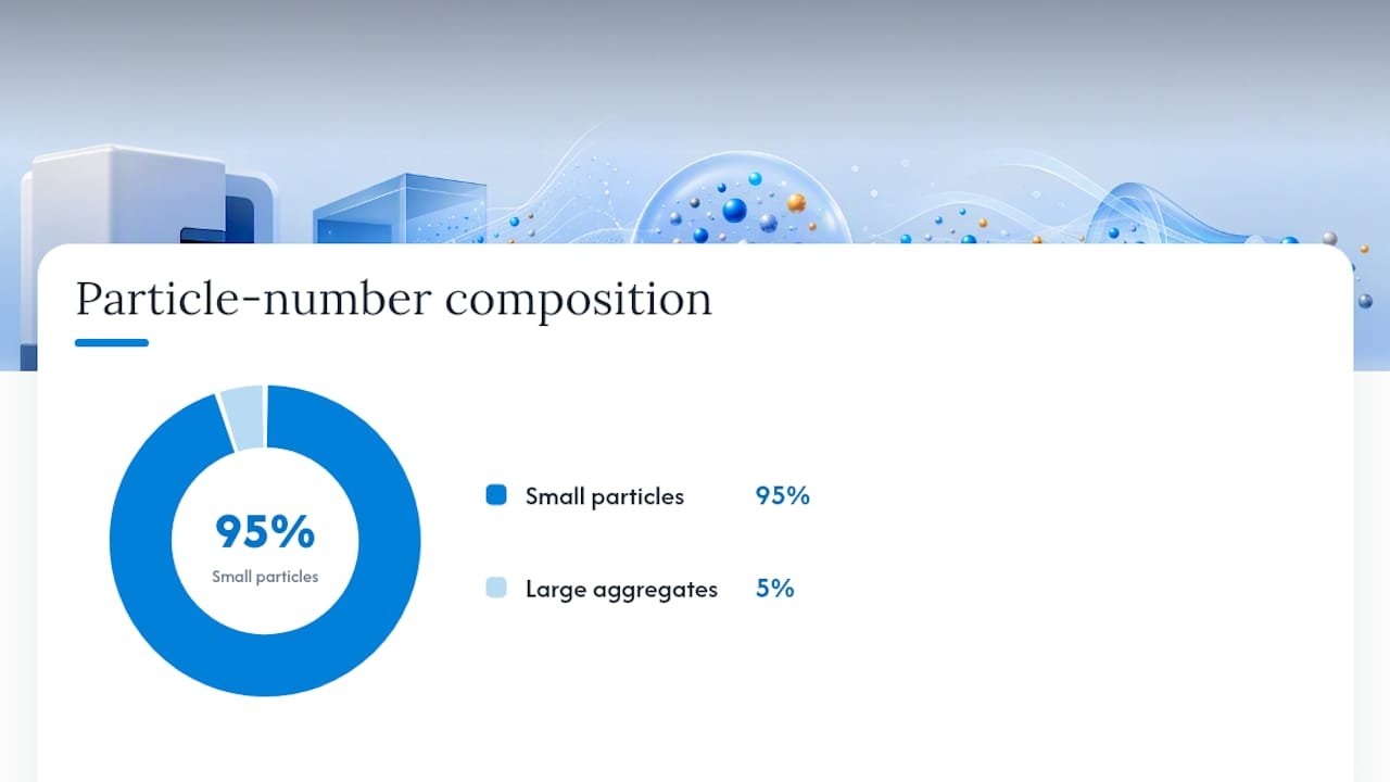
That difference has real practical consequences. A sample that is 95% small particles and 5% large aggregates by number will show DLS results skewed heavily toward the aggregate size, since those few large particles scatter far more light than the many small ones. NTA, because it counts particles individually rather than weighting by scattered intensity, will correctly show the aggregates as a small distinct population sitting on top of the dominant small-particle peak.

Sensitivity and speed cut the other way. DLS instruments are generally faster to run, need less sample prep, and give a usable mean size in minutes on genuinely monodisperse samples. NTA needs a video acquisition, particle-by-particle tracking, and more careful dilution to get particles into a countable range, which takes longer per sample.

A few situations make the choice fairly clear:

• Reach for NTA when you suspect aggregates, need a true concentration value, or are characterizing a heterogeneous population like extracellular vesicles or a lipid nanoparticle formulation with minor subpopulations.
• Reach for DLS when you have a genuinely monodisperse sample and just need a fast mean-size check for batch-to-batch quality control.
• Run both when the sample matters enough to publish or file a regulatory submission on. NTA’s number-based resolution and concentration data pair well with DLS’s speed and its sensitivity to the earliest signs of aggregation, and combining the two techniques gives a fuller characterization than either alone.

Neither technique replaces the other completely. Labs that treat NTA and DLS as competing options rather than complementary ones tend to miss real changes in their formulations.

What Instrument Modes Does NTA Offer?

Most NTA instruments run in two modes, and the choice between them depends entirely on what question you’re actually asking about the sample.

Scattering mode is the default: the laser illuminates everything in the field of view, and every particle above the detection threshold gets tracked and sized regardless of what it’s made of. This is fast, requires no sample labeling, and works for straightforward size and concentration questions on liposomes, synthetic nanoparticles, or unlabeled protein aggregates.

Fluorescence mode adds a filter that blocks scattered laser light and only passes emission from fluorescently labeled particles. This lets you count and size a specific subpopulation, such as extracellular vesicles carrying a particular surface marker, inside a mixed or biologically complex sample where scattering mode would just show you everything at once with no way to distinguish targets from background debris. Fluorescence NTA depends heavily on labeling efficiency, dye choice, and instrument sensitivity; a poorly optimized label gives you a dim, unreliable signal no amount of software tweaking will fix.

A few hardware and setup considerations affect how well either mode performs:

• Laser wavelength selection needs to match your fluorophore’s excitation spectrum and avoid excessive overlap with autofluorescence in biological samples.
• Camera exposure and gain control how much signal you capture per frame; too high introduces noise and false tracks, too low misses dim particles.
• Flow cell versus static cuvette setups trade continuous sample delivery (better for concentration precision over longer captures) against simplicity and lower sample volume requirements.
• Regular calibration against certified size standards (commonly polystyrene or silica beads of known diameter) confirms the optical path and tracking algorithm are performing as expected before you trust results on an unknown sample.

Pro Tip: If you’re deciding whether fluorescence NTA is worth the extra setup time, ask whether your research question depends on identifying a specific subpopulation within a mixed sample. If you just need total particle size and count, scattering mode is faster and has one less variable to troubleshoot.

What Sample Prep and Settings Give Reproducible Results?

Reproducible NTA data starts before the sample ever reaches the instrument. Getting consistent, publishable numbers means controlling a short list of variables that most protocol failures trace back to.

1. Filter or clean up the sample to remove large debris and bubbles before dilution. A pre-filtration step (commonly through a membrane in the sub-0.02 micron range for buffer or diluent) removes contaminating particles that would otherwise show up as false signal.
2. Dilute to the correct working concentration. Aim for roughly 10 to 50 particles visible per frame, which generally corresponds to a working concentration in the range of 10^8 to 10^9 particles per milliliter. Too concentrated and tracks overlap, corrupting trajectories; too dilute and you don’t collect enough particles for statistically meaningful counts.
3. Set the detection threshold carefully. Published protocols point to a threshold setting of approximately 5 as a reasonable operational target in many systems, high enough to exclude background noise but low enough to still catch genuine dim particles.
4. Fix camera level and gain at values that show particles clearly without diffractive rings or overexposed halos, and document those exact settings.
5. For flow-cell setups, control flow rate so particles move through the imaging volume at a speed the tracking algorithm can follow reliably without introducing motion blur.
6. Capture multiple video replicates, not just one. This is the step most labs shortcut, and it’s the one with the clearest evidence behind it.

Increasing replicate count matters more than most researchers assume. Work specifically testing NTA concentration precision in biofluids found that increasing video replicates from 5 up to 15 or 25 measurably reduces variance and relative standard error, particularly for particles in the 50 to 120 nanometer range common to extracellular vesicle work. A single video, however carefully captured, simply doesn’t sample enough particles to give you a stable concentration estimate.

Pro Tip: Treat your concentration number with more skepticism than your size number. Sizing tends to be robust once the optics are set correctly, but concentration is the output most vulnerable to dilution error, particle-per-frame miscounts, and insufficient replicates. When in doubt, run more videos rather than trusting one.

Build a simple checklist into your lab notebook template so these settings get recorded every time, not just when someone remembers:

• Instrument model and software version
• Laser wavelength and mode (scattering or fluorescence)
• Dilution factor and final working concentration estimate
• Camera level, gain, and detection threshold values
• Number of video replicates and capture duration per replicate
• Calibration standard used and date of last calibration check

How Should You Interpret and Report NTA Data?

NTA output is a number-weighted histogram, typically binned in nanometer increments, showing particle count against hydrodynamic diameter. Reading it correctly means remembering it counts particles, not mass or scattering intensity, so a tall narrow peak at 100 nanometers with a small bump at 400 nanometers means many small particles and comparatively few large ones, even if that small bump looks visually significant on the chart.

A few artifacts show up often enough that you should know them by sight. Overexposure produces diffractive rings around particles that can be mistakenly tracked as separate objects, inflating apparent concentration. Overlapping tracks at high concentration cause the algorithm to lose or merge trajectories, corrupting both size and count. Contaminating particles, dust, or air bubbles introduce false positives that shift the whole distribution, particularly at the small end where debris and true nanoparticles can be hard to distinguish visually.

Precision reporting separates a rigorous NTA dataset from a sloppy one. Running multiple video replicates lets you calculate relative standard error (RSE) or root-mean-square error (RMSE) across those replicates rather than reporting a single-video number with no error bar at all. Sizing accuracy under correctly calibrated conditions typically falls within about 5% of the expected particle diameter, a benchmark worth stating explicitly in methods sections so reviewers know your setup was validated against known standards rather than assumed.

For a methods section that would survive peer review, include:

• Instrument make, model, and software version
• Laser wavelength and detection mode used
• Camera level, gain, and detection threshold
• Dilution scheme and calculated working concentration
• Number of video replicates, frame rate, and capture duration per replicate
• Calibration standard and verification date

Reported sizing accuracy: Properly calibrated NTA systems achieve sizing accuracy within roughly 5% of expected particle diameter when settings are validated against certified size standards, a figure worth citing directly when justifying your methodology to reviewers or auditors.

Where Does NTA Add the Most Value?

Extracellular vesicle (EV) and exosome research is where NTA has become close to a default technique, largely because EV preparations are polydisperse and concentration matters as much as size for downstream dosing calculations. Fluorescence-mode NTA extends this further, letting researchers confirm phenotype by counting only particles carrying a specific membrane marker rather than every scattering object in a crude EV prep, though that approach is only as reliable as the labeling strategy behind it. Complex biofluids like plasma or cerebrospinal fluid introduce their own problem: background particles and lipoprotein contamination can swamp the true EV signal, which means results from unpurified biofluids need cautious interpretation.

Lipid nanoparticle (LNP) and vaccine adjuvant formulation work leans on NTA for a different reason: batch consistency. Formulation scientists track size distribution and concentration across production runs to catch drift early, since a shift in either metric often signals a process problem upstream.

Protein aggregation studies use NTA to catch what bulk techniques miss: a small population of aggregates forming in an otherwise stable formulation, visible as a distinct minor peak well before it would show up as a meaningful shift in a DLS Z-average.

Common application areas where NTA earns its place in the workflow:

• Extracellular vesicle and exosome quantitation, including fluorescent phenotyping of marker-positive subpopulations
• Lipid nanoparticle and vaccine adjuvant characterization during formulation development and batch QC
• Protein aggregate detection in stability and shelf-life studies
• Viral particle and synthetic nanoparticle sizing across research and process development

For regulatory submissions or high-stakes publications, pair NTA with an orthogonal method such as transmission electron microscopy (TEM) for direct morphology, or resistive pulse sensing (RPS) for an independent concentration check. No single technique should carry that much weight alone.

What Common Mistakes Undermine NTA Data?

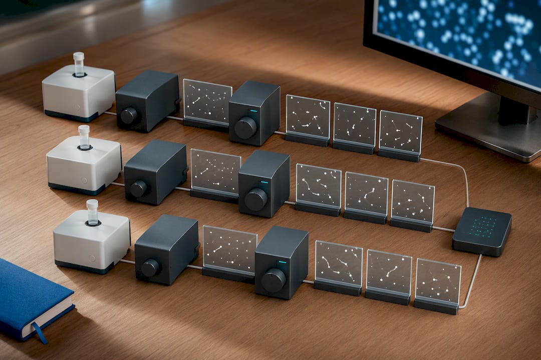
Operator-adjusted settings are the biggest source of irreproducibility in NTA data, full stop. Detection threshold and camera level are subjective calls unless a lab enforces a written SOP, and two operators running the same sample with different threshold choices can generate meaningfully different concentration numbers from identical raw video. Document every setting, every time, and don’t let “the software’s default” substitute for a deliberate, recorded choice.

Refractive index dependence catches researchers who assume NTA gives an absolute size measurement. It doesn’t; it gives a hydrodynamic diameter, a spherical equivalent based on diffusion behavior. Non-spherical or low-refractive-index particles will size differently on NTA than on TEM or RPS, and that divergence is expected physics, not instrument error.

Concentration precision degrades badly at low particle counts, where statistical noise dominates. The fix isn’t a software trick, it’s methodology: dilute into the recommended particles-per-frame range, and run enough video replicates that a single unlucky capture doesn’t define your reported number.

• Enforce a written SOP for detection threshold and camera settings across all operators
• Never report hydrodynamic diameter as an absolute measurement for non-spherical particles without a caveat
• Increase replicate count rather than trusting a single low-count video
• Recognize when NTA isn’t the right tool: samples below roughly 10 nanometers, highly concentrated undiluted samples, or matrices with heavy background contamination may need a different technique entirely

Pro Tip: If your concentration numbers vary wildly between technical replicates on the same sample, check particles-per-frame first before blaming the instrument. Nine times out of ten it’s a dilution or threshold problem, not a hardware fault.

Mayflowerbio’s Nanoparticle Tracking Analysis Services

Mayflowerbio offers NTA size profiling as a specialized service for labs that need reliable size distribution and concentration data without building out in-house instrumentation and SOPs from scratch. Standard deliverables include a full size distribution histogram, a concentration measurement with replicate-based precision reporting, and complete methods metadata documenting instrument settings, calibration status, and acquisition parameters, ready to drop into a manuscript or regulatory file.

For labs working through the full EV or vesicle pipeline, complementary product lines support the upstream and downstream steps NTA depends on:

• Exosome isolation reagents and kits for clean starting material before sizing
• Exosome detection reagents for fluorescence-mode labeling and phenotype confirmation
• Purified exosomes as reference material for method validation and instrument calibration checks

Labs building a new protocol or troubleshooting inconsistent results can request the NTA size profiling service directly or reach out for protocol consultation before committing to an in-house setup.

A Minimum Reporting Standard Worth Enforcing

If I had to compress everything above into one insistence, it’s this: report your settings or your data isn’t reproducible, full stop. Every NTA paper or QC record should state the instrument model, laser wavelength, camera level and gain, detection threshold, number of video replicates, and particles-per-frame at acquisition. Skip any one of those and a different lab cannot tell whether their diverging result is real biology or just a different threshold setting. This isn’t bureaucratic box-checking; it’s the difference between data anyone can trust and a number nobody can reproduce. If your lab needs help building that workflow, Mayflowerbio’s team can walk through protocol design or run the profiling directly.

— Alina

Get Reproducible NTA Data Without Building It In-House

Running NTA correctly means owning a laser-based instrument, writing enforceable SOPs, training every operator on identical settings, and still budgeting for calibration standards and replicate captures on every sample. Mayflowerbio’s NTA size profiling service gives labs that same rigor, size distribution, concentration with replicate-based precision, and full methods metadata, without the capital cost or the months of SOP development.

This fits particularly well for labs running extracellular vesicle, lipid nanoparticle, or protein aggregation work who need publication-ready data on a project timeline rather than an instrument-validation timeline. It also pairs naturally with Mayflowerbio’s exosome isolation and detection reagents for labs handling the full EV workflow from raw sample to final size report. If your next manuscript or regulatory filing needs sizing and concentration data with real precision reporting behind it, explore the bioassay and reagent catalog or request the NTA profiling service to get a quote and discuss your sample type before you commit to a timeline.

Sources

• Critical parameters to standardize size and concentration determination by NTA — PubMed
• Comparisons between NTA and DLS approaches (PMC review)
• Nanoparticle Tracking Analysis: An Effective Tool to Characterize Extracellular Vesicles — MDPI review
• Synergy of complementary nanomaterial characterization techniques — Malvern Panalytical whitepaper

FAQ

What Is the Difference Between DLS and NTA?

DLS reports an intensity-weighted average size across the whole particle ensemble, so larger particles dominate the signal disproportionately, while NTA tracks individual particles and reports a number-weighted distribution plus a direct concentration measurement DLS cannot provide.

What Instrument Is Used for Nanoparticle Tracking Analysis?

NTA instruments combine a laser light source, a flow cell or static cuvette to hold the sample, and a camera that records particle scattering (or fluorescence) on video for software-based tracking and sizing.

How Does Nanoparticle Tracking Analysis Work, Exactly?

The instrument films particles undergoing Brownian motion, tracks each one’s movement across frames, and uses the Stokes–Einstein equation to convert that diffusion behavior into a hydrodynamic diameter for every particle individually.

What Is Nanoparticle Analysis Used For?

It’s used to measure size distribution and absolute concentration of nanoparticles in a sample, most commonly for extracellular vesicles, lipid nanoparticles and vaccine adjuvants, and protein aggregates during formulation and stability studies.

How Many Video Replicates Should You Capture for Reliable NTA Data?

Evidence specifically testing concentration precision found that increasing replicates from 5 to 15 or 25 meaningfully reduces variance, so most labs should plan for at least that range rather than relying on a single video capture.

Recommended

• Nanotechnology Company Guide for Biomedical Researchers
• NTA Size Profiling Service